Not how it works, you can easily read original research or some source code for that, but the why. Why does Markov Chain Monte Carlo sampling work?

I’ll start by introducing the idea of a probability density function. Everyone is familiar with six-sided dice, yes? There are two ways to figure out the odds of rolling a specific face: manually roll the die multiple times and use the totals as a prediction, or invoke a bit of information theory. The latter sounds scary, but is actually quite intuitive. We know there are six faces and thus six possible outcomes, and only one of them will be chosen. We have no justification for thinking one is more likely than the other, so they must all be equally likely. Therefore they must each have ¹/₆th of the total probability, ergo the probability is ¹/₆. By wrapping this all into a program and then charting the output, we see that both methods come to the same conclusion.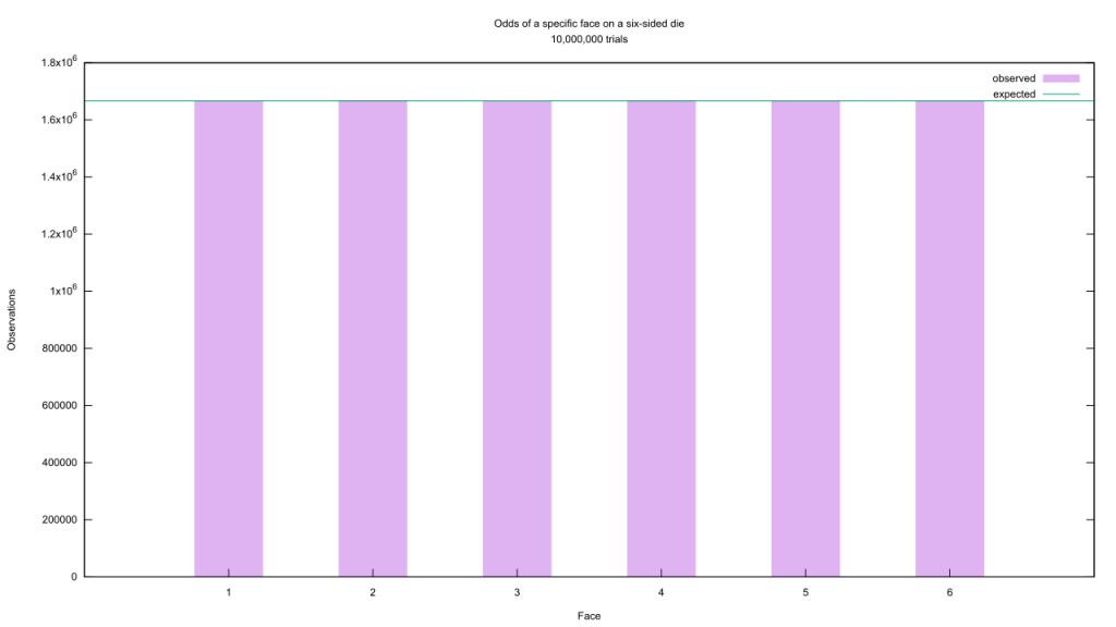Yawn. Let’s raise the difficulty a bit, then, and swap the six-sided die for the random number generator I used to simulate it. This creates a problem, as in theory there are now 2³² possible outcomes instead of 6. We can’t chart that many categories! Instead, we can group them together into bins and chart the number of values that fell into each bin. With the help of another program and another chart, we see a pattern emerge.

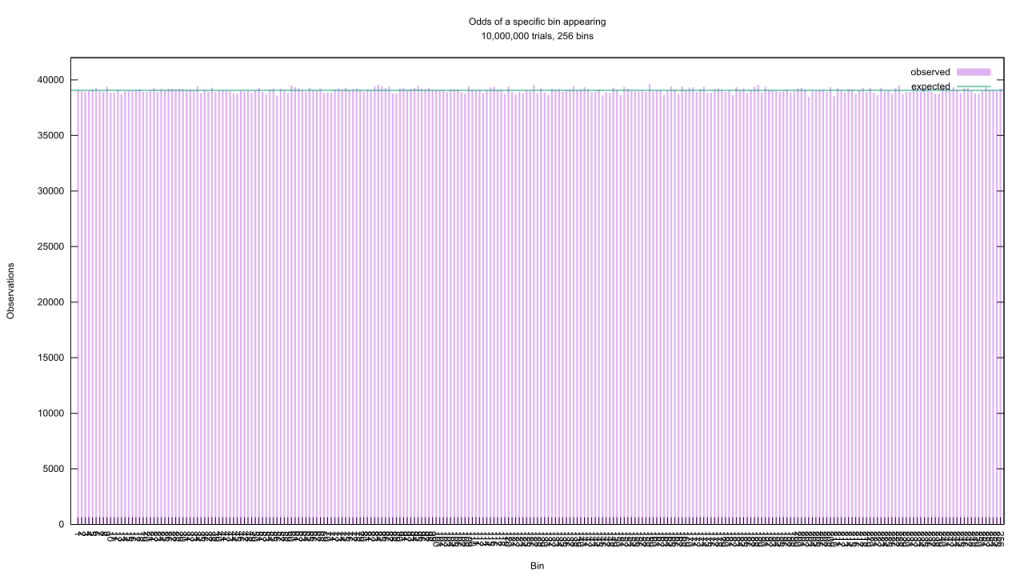As we group the output of this random number generator into more and more bins, the number of observations in each bin fluctuates more and more but still clusters around a flat expected value. This makes sense, as the same logic we used to determine how often each face of a six-sided die would come up applies here: this is a uniform random number generator that churns out values between 0 and 1, which means that any value it returns is equally as likely as any other.

Wouldn’t it be handy if we had a function which takes in one of those random numbers and gives back how likely it is to appear? We could calculate an integral of this probability density function if we want to know the likelihood for a given range of numbers, too. In the case of a uniform random number generator, we know that the derivative of this function is zero everywhere (otherwise, one value would be more likely than another). We also know that it can only return values between 0 and 1, therefore the odds of getting a value from that range are 100%, therefore the integral of that range equals one.

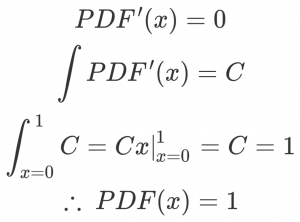There! To find the likelihood of getting a random number in a range, we only need to evaluate the integral of the PDF between the two points; for instance, the odds of getting a random number between ¹/₆ and ⁵/₆ is ⁵/₆ – ¹/₆ = ²/₃. Since it shows up so often, the integral of the PDF has a shorter name: the cumulative distribution function, or CDF to its friends.

We can turn up the difficulty even more by looking at biased random number generators. Imagine throwing multiple dice instead of one, and using the sum of what comes up. As the number of dice increases, the likelihood of outcomes begins to cluster around a single value; there are six ways to roll a seven with two dice (1 and 6, 2 and 5, and so on), while there’s only one way to roll a two, so the former will appear six times more often than the latter. Keep piling on the dice, and the overall distribution trends towards a familiar shape. We can simulate this shape, too.

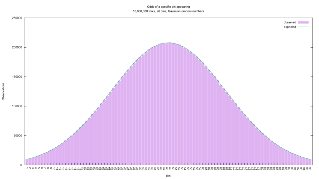That’s the infamous “bell curve” or Gaussian/normal distribution. The formula to describe its probability density function is a bit trickier than the previous, and the CDF formula is, well…

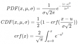… something. More to the point, nothing’s really changed from the uniform random number distribution: we have a function which predicts how likely any given value will be, as well as an integral of it which allows us to calculate the odds of the output falling into a range. The bias in outcomes only makes the math a bit trickier. So let’s examine a third random number distribution which is somewhere between those two.

Staircase functions are old hat, but I’ve searched and been unable to find anyone else defining this “Geometric Staircase.” Each step on the Staircase is exactly half the width of the previous one, as well as half the height. That isn’t obvious from the programming code, because it was buried under the dancing I needed to do to calculate the CDF and its inverse. Interesting fact: if you can lay your hands on the inverse of a CDF, you can transform a uniform random number generator into a biased one which follows the contours of the associated PDF.

The area under the graph is governed by the geometric sum

and since that sums to 1, it’s trivial to calculate the area of each step and therefore the odds of a random number appearing on it.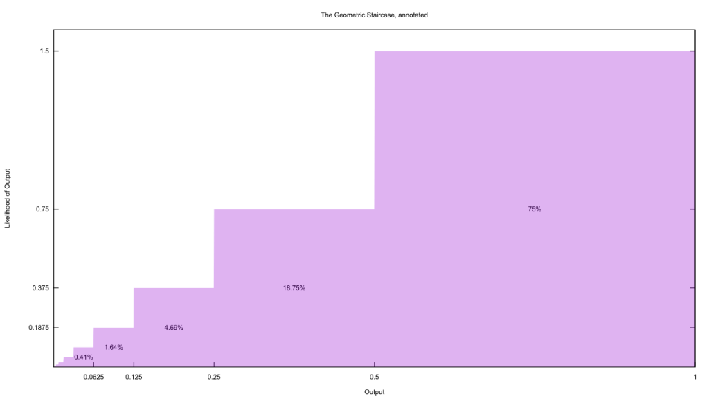That top-most stair contains 75% of all emitted random numbers, the next contains a quarter of that or about 18.75%, and so on down the line.

Now brace yourself, because things are about to get even cooler. Not only do we have three random number generators, we have a way to verify they behave as expected: sort their output into bins and use the CDF to examine the totals. If any number-generating algorithm gives an output that matches the PDF/CDF, it is functionally identical to the corresponding random number generator.

I think you can guess what’ll happen next.

If I code up a simple Metropolis MCMC sampler and feed it any one of those three PDFs, its output will resemble that of the associated random number generator! The more I iterate on my samples, the closer that resemblance becomes. This is true for any other MCMC algorithm, which means all of them are, in essence, crummy random number generators. I say “crummy” because of their heavy computational cost.

	Uniform	Gaussian	Geometric Staircase
RNG	22.8	38.2	31.3
MCMC	11152.0	30846.0	16254.0
(nanosecond per value output, median of 5 trials, 20 sample MCMC)

However, those same MCMC algorithms are also ridiculously flexible random number generators. The only reason I included CDFs in their code was to evaluate their performance, the output of MCMC depends only on the PDF. The latter is a lot easier to create, believe me, so for complicated distributions it’s MCMC or bust. If you look carefully, you’ll also notice I’m not using the proper PDFs for the Gaussian or Geometric Staircase examples; since the main driver of MCMC algorithms is relative likelihood, any constant scaling factor is redundant and can be omitted without changing the results.

What sorcery is this?! The magic happens during the decision part of the algorithm. For my simple Metropolis MCMC, the likelihood of a new candidate is compared to the likelihood of the sample it could replace. If the new one is more likely, it wins by default. Scroll up to the Geometric Staircase graph and picture a point on the far left. As we draw random samples from along the bottom of the graph, there’s a good chance we’ll run across one sitting on a higher stair. If that was the entire decision rule, the net effect would be to bounce up the staircase to the top.

It’s not, however. Even if the new candidate is less likely, there’s another way it could replace the old sample. We draw from a uniform random number generator, and compare that value to the proportion between the new and old likelihoods. If the random number is smaller than the proportion, we replace the old with the new anyway. Suppose the old value is a point on the top stair: that is twice the height of the next stair down, so there’s a 50% chance that we’d jump to a new candidate sitting on the lower stair. Since the width of that stair is also half of the current one, we’re half as likely to draw a new candidate from that stair as we are from the same stair we’re sitting on. The net effect is that from a point on that top stair, there’s a 25% chance we’ll jump down one step. Similar logic determines we have a 6.25% chance of jumping down two steps, and so on down the staircase. Once our sample reaches the top of the stair, then, where it hops next precisely mirrors the contours of the PDF. It behaves as if it was the output of the matching random number generator.

This also explains why Bayesian statistics has gone ga-ga for MCMC. On that side of the fence, almost everything is a probability distribution. Any possible value for a parameter of any hypothesis has a likelihood attached to it, and when collected together they form a PDF. Tossing MCMC at the parameters of a hypothesis will give you a random sample from their PDFs; if a lucky few of them are very likely given the evidence, the result will be a tight cluster of samples around a few values. Conversely, if a wide range of parameters are compatible with what we observe, the samples will be spread out and reflect the underlying uncertainty around the real-life value of the parameter.

Let’s put that to the test with one of my favorite examples: Jaynes’ Truncated Exponential.

The following problem has occurred in several industrial quality control situations. A device will operate without failure for a time θ because of a protective chemical inhibitor injected into it; but at time θ the supply of the chemical is exhausted, and failures then commence, following the exponential failure law. It is not feasible to observe the depletion of this inhibitor directly; one can observe only the resulting failures. From data on actual failure times, estimate the time θ of guaranteed safe operation …

Jaynes, Edwin T., and Oscar Kempthorne. “Confidence intervals vs Bayesian intervals.” Foundations of probability theory, statistical inference, and statistical theories of science. Springer, Dordrecht, 1976. Pg. 196-201

The above chart shows off the PDF for how these parts fail. The part below the half-way mark isn’t small, it’s exactly zero, and that has important consequences. If we guess a value of θ which is higher than any part’s failure time, the likelihood of that guess matching reality is zero. Conversely, any value of θ less than every observed failure time has a likelihood greater than zero, although the gentle slouch towards the x-axis implies that the earlier we move θ relative to the earliest failure, the less likely that θ matches reality. Just by thinking out loud we can work out that the PDF of θ likelihoods is roughly the mirror image of the failure PDF, with a tail that starts at the origin then rises up to peak at the first failure point, and drops straight to zero after that point.

Frequentist statistics doesn’t have the concept of parameter likelihoods, however, and takes a very different approach to this problem. Jaynes himself has a good write-up with math behind both, though I’ll confess I first learned about it over here. My implementation of both the frequentist and Bayesian approaches is here.

The frequentist answer on the left is obviously wrong. With only one observation as input, the most probable failure point is quite a bit earlier than we expect (sneak a peek at the matching Bayesian answer). The confidence interval gives almost no credence to early failure points, even though they’re quite plausible when we’ve only looked at a single sample. While the sharp falloff makes it difficult to tell, frequentism assigns a Gaussian distribution to the failure point’s confidence interval, which also means it assigns a non-zero likelihood for values of θ after the earliest failure. It should get better as we feed more observations in, but thanks to a limited sample size and some bad RNG a whopping 70 to 91% of the credible interval is after the earliest failure! That mysterious black vertical line is the ground truth value, and as you can see frequentism only nailed it for N = 3.

Compare that to the Bayesian answer, which invoked MCMC. With N = 1, the PDF of θ behaves exactly as we guessed it should. As we pile on the evidence, the tail gets steeper and steeper while the maximal likelihood of the PDF inches closer to the ground truth value. We see the promised transition from a wide range of likely parameters to a narrow one as our certainty increases, and unlike the frequentist method we quickly converge on the ground truth.

This, I hope, hammers home the “why” of MCMC: it is a highly-customizable random number generator, thanks to a clever bit of math. Certain tasks are a lot easier with such generators, like Bayesian statistics, and the speed of computers defangs their heavy computational cost. Ergo why MCMC algorithms are used so often and studied so intently.