Feeling the Research

Daryl Bem must be sick of those puns by now.

Back in 2011 he published Feeling the Future, a paper that combined multiple experiments on human precognition to argue it was a thing. Naturally this led to a flurry of replications, many of which riffed on his original title. I got interested via a series of blog posts I wrote that, rather surprisingly, used what he published to conclude precognition doesn’t exist.

I haven’t been Bem’s only critic, and one that’s a lot higher profile than I has extensively engaged with him both publicly and privately. In the process, they published Bem’s raw data. For months, I’ve wanted to revisit that series with this new bit of data, but I’m realising as I type this that it shouldn’t live in that Bayes 20x series. I don’t need to introduce any new statistical tools to do this analysis, for starters; all the new content here relates to the dataset itself. To make understanding that easier, I’ve taken the original Excel files and tossed them into a Google spreadsheet. I’ve re-organized the sheets in order of when the experiment was done, added some new columns for numeric analysis, and popped a few annotations in.

Odd Data

The first thing I noticed was that the experiments were not presented in the order they were actually conducted. It looks like he re-organized the studies to make a better narrative for the paper, implying he had a grand plan when in fact he was switching between experimental designs. This doesn’t affect the science, though, and while never stating the exact order Bem hints at this reordering on pages three and nine of Feeling the Future.

What may affect the science are the odd timings present within many of the datasets. As Dr. R pointed out in an earlier link, Bem combined two 50-sample studies together for the fifth experiment in his paper, and three studies of 91, 19, and 40 students for the sixth. Pasting together studies like that is a problem within frequentist statistics, due to the “stopping problem.” Stopping early is bad, because random fluctuations may blow the p-value across the “statistically significant” line when additional data would have revealed a non-significant result; but stopping too late is also bad, because p-values tend to exaggerate the evidence against the null hypothesis and the problem gets worse the more data you add.

But when pouring over the datasets, I noticed additional gaps and oddities that Dr. R missed. Each dataset has a timestamp for when subjects took the test, presumably generated by the hardware or software. These subjects were undergrad students at a college, and grad students likely administered some or all the tests. So we’d expect subject timestamps to be largely Monday to Friday affairs in a continuous block. Since these are machine generated or copy-pasted from machine-generated logs, we should see a monotonous increase.

Yet that 91 study which makes up part of the sixth study has a three-month gap after subject #50. Presumably the summer break prevented Bem from finding subjects, but what sort of study runs for a month, stops for three, then carries on for one more? On the other hand, that logic rules out all forms of replication. If the experimental parameters and procedure did not change over that time-span, either by the researcher’s hand or due to external events, there’s no reason to think the later subjects differ from the former.

Look more carefully and you see that up until subject #49 there were several subjects per day, followed by a near two-week pause until subject #50 arrived. It looks an awful like Bem was aiming for fifty subjects during that time, was content when he reached fourty-nine, then luck and/or a desire for even numbers made him add number fifty. If Bem was really aiming for at least 100 subjects, as he claimed in a footnote on page three of his paper, he could have easily added more than fifty, paused the study, and resumed in the fall semester. Most likely, he was aiming for a study of fifty subjects back then, suggesting the remaining forty-one were originally the start of a second study before later being merged.

Experiment 1, 2, 4, and 7 also show odd timestamps. Many of these can be explained by Spring Break or Thanksgiving holidays, but many also stop at round numbers. There’s also instances where some timestamps occur out-of-order or the sequence number reverses itself. This is pretty strong evidence of human tampering, though “tampering” isn’t the synonymous with “fraud;” any sufficiently large study will have mistakes, and any attempt to correct those mistakes will look like fraud. That still creates uncertainty in a dataset and necessarily lowers our trust in it.

I’ve also added stats for the individual runs, and some of them paint an interesting tale. Take experiment 2, for instance. As of the pause after subject #20, the success rate was 52.36%, but between subject #20 and #100 it was instead 51.04%. The remaining 50 subjects had a success rate of 52.39%, bringing the total rate up to 51.67%. Why did I place a division between those first hundred and last fifty? There’s no time-stamp gap there, and no sign of a parameter shift. Nonetheless, if we look at page five and six of the paper, we find:

For the first 100 sessions, the flashed positive and negative pictures were independently selected and sequenced randomly. For the subsequent 50 sessions, the negative pictures were put into a fixed sequence, ranging from those that had been successfully avoided most frequently during the first 100 sessions to those that had been avoided least frequently. If the participant selected the target, the positive picture was flashed subliminally as before, but the unexposed negative picture was retained for the next trial; if the participant selected the nontarget, the negative picture was flashed and the next positive and negative pictures in the queue were used for the next trial. In other words, no picture was exposed more than once, but a successfully avoided negative picture was retained over trials until it was eventually invoked by the participant and exposed subliminally. The working hypothesis behind this variation in the study was that the psi effect might be stronger if the most successfully avoided negative stimuli were used repeatedly until they were eventually invoked.

So precisely when Bem hit a round number and found the signal strength was getting weaker, he tweaked the parameters of the experiment? That’s sketchy, especially if he peeked at the data during the pause at subject #20. If he didn’t, the parameter tweak is easier to justify, as he’d already hit his goal of 100 subjects and had time left in the semester to experiment. Combining both experimental runs would still be a no-no, though.

Uncontrolled Controls

Bem’s inconsistent use of controls was present in the paper, but it’s a lot more obvious in the dataset. In experiments 2, 3, 4, and 7 there is no control group at all. That is dangerous. If you run a control group through a protocol nearly identical to that of the experimental group, and you don’t get a null result, you’ve got good evidence that the procedure is flawed. If you don’t run a control group, you’d better be damn sure your experimental procedure has been proven reliable in prior studies, and that you’re following the procedure close enough to prevent bias.

Bem doesn’t hit that for experiments 2 and 7; the latter isn’t the replication of a prior study he’s carried out, and while the former is a replication of experiment 1 the earlier study was carried out two years before and appears to have been two separate sample runs pasted together, each with different parameters. In experiments 3 and 4, Bem’s comparing something he knows will have an effect (forward priming) with something he hopes will have an effect (retroactive priming). There’s no explicit comparison of the known-effect’s size to that found in other studies, Bem’s write-up appears to settle for showing statistical significance. Merely showing there is an effect does not demonstrate that effect is of the same magnitude as expected.

Conversely, experiments 5 and 6 have a very large number of controls, relative to the experimental conditions. This is wasteful, certainly, but it could also throw off the analysis: since the confidence interval narrows as more samples are taken, we can tighten one side up by throwing more datapoints in and taking advantage of the p-value’s weakness.

Experiment 6 might show this in action. For the first fifty subjects, the control group was further from the null value than the negative image group, but not as extreme as the erotic image one. Three months later, the next fourty-one subjects are further from the null value than both the experimental groups, but this time in the opposite direction! Here, Bem drops the size of the experimental groups and increases the size of the control group; for the next nineteen subjects, the control group is again more extreme than the negative image group and again less extreme than the erotic group, plus the polarity has flipped again. For the last fourty subjects, Bem increased the sizes of all groups by 25%, but the control is again more extreme and the polarity has flipped yet once more. Nonetheless, adding all four runs together allows all that flopping to cancel out, and Bem to honestly write “On the neutral control trials, participants scored at chance level: 49.3%, t(149) = -0.66, p = .51, two-tailed.” This looks a lot like tweaking parameters on-the-fly to get a desired outcome.

It also shows there’s substantial noise in Bem’s instruments. What’s the odds that the negative image group success rate would show less variance than the control group, despite having anywhere from a third to a sixth of the sample size? How can their success rate show less variance than the erotic image group, despite having the same sample size? These scenarios aren’t impossible, but with them coming at a time when Bem was focused on precognition via negative images it’s all quite suspicious.

The Control Isn’t a Control

All too often, researchers using frequentist statistics get blinded by the way p-values ignore the null hypothesis, and don’t bother checking their control groups. Bem’s fairly good about this, but we can do better.

All of Bem’s experiments, save 3 and 4, rely on Bernoulli processes; every person has some probability of guessing the next binary choice correctly, due possibly to inherent precognitive ability, and that probability does not change with time. It follows that the distribution of successful guesses follows the binomial distribution, which can be written:

P( s `divides` p,f ) ~=~ { (s+f)"!" } over { s"!" f"!" } p^s ( 1-p )^f where s is the number of successes, f the number of failures, and p the odds of success; that means P ( s | p,f ) translates to “the probability of having s successes, given the odds of success are p and there were f failures.” Naturally, p must be between 0 and 1.

Let’s try a thought experiment: say you want to test if a single six-sided die is biased to come up 1. You roll it thirty-six times, and observe four instances where it comes up 1. Your friend tosses it seventy-two times, and spots fifteen instances of 1. You’d really like to pool your results together and get a better idea of how fair the die is; how would you do this? If you answered “just add all the successes together, as well as the failures,” you nailed it!The probability distribution of rolling a 1 for a given die, according to you and your friend's experiments.
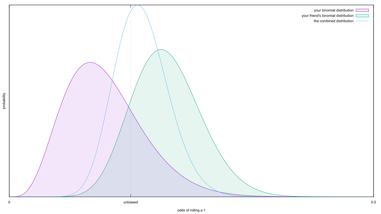
The results look pretty good; both you and your friend would have suspected the die was biased based on your individual rolls, but the combined distribution looks like what you’d expect from a fair die.

But my Bayes 208 post was on conjugate distributions, which defang a lot of the mathematical complexity that comes from Bayesian methods by allowing you to merge statistical distributions. Sit back and think about what just happened: both you and your friend examined the same Bernoulli process, resulting in two experiments and two different binomial distributions. When we combined both experiments, we got back another binomial distribution. The only way this differs from Bayesian conjugate distributions is the labeling; had I declared your binomial to be the prior, and your friend’s to be the likelihood, it’d be obvious the combination was the posterior distribution for the odds of rolling a 1.

Well, almost the only difference. Most sources don’t list the binomial distribution as the conjugate for this situation, but instead the Beta distribution:

Beta( p `divides` %alpha,%beta ) ~=~ { %GAMMA(%alpha + %beta) } over { %GAMMA(%alpha) %GAMMA(%beta) } p^{%alpha-1} ( 1-p )^{%beta-1}

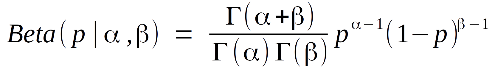
But I think you can work out the two are almost identical, without any help from me. The only real advantage of the Beta distribution is that it allows non-integer successes and failures, thanks to the Gamma function, which in turn permits a nice selection of priors.

In theory, then, it’s dirt easy to do a Bayesian analysis of Bem’s handiwork: tally up the successes and failures from each individual experiment, add them together, and plunk them into a binomial distribution. In practice, there are three hurdles. The easy one is the choice of prior; fortunately, Bem’s datasets are large enough that they swamp any reasonable prior, so I’ll just use the Bayes-Laplace one and be done with it. A bigger one is that we’ve got at least three distinct Bernoulli processes in play: pressing a button to classify an image (experiments 3, 4), remembering a word from a list (8, 9), and guessing the next image out of a binary pair (everything else). If you’re trying to describe precognition and think it varies depending on the input image, then the negative image trials have to be separated from the erotic image ones. Still, this amounts to little more than being careful with the datasets and thinking hard about how a universal precognition would be expressed via those separate processes.

The toughest of the bunch: Bem didn’t record the number of successes and failures, save experiments 8 and 9. Instead, he either saved log timings (experiments 3 and 4) or the success rate, as a percentage of all trials. This is common within frequentist statistics, which is obsessed with maximal likelihoods, but it destroys information we could use to build a posterior distribution. Still, this omission isn’t fatal. We know the number of successes and failures are integer values. If we correctly guess their sum and multiply it by the rate, the result will be an integer; if we pick an incorrect sum, it’ll be a fraction. A complication arrives if there are common factors between the number of successes and the total trials, but there should some results which lack those factors. By comparing results to one another, we should be able to work out both what the underlying total was, as well as when that total changes, and in the process we learn the number of successes and can work backwards to the number of failures.

As the heading suggests, there’s something interesting hidden in the control groups. I’ll start with the binary image pair controls, which behave a lot like a coin flip; as the samples pile up, we’d expect the control distribution to migrate to the 50% line. When we do all the gathering, we find…

What happens when we combine the control groups for the binary image process from Bem (2011).
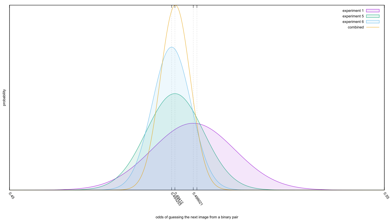
… that’s not good. Experiment 1 had a great control group, but the controls from experiment 5 and 6 are oddly skewed. Since they had a lot more samples, they wind up dominating the posterior distribution and we find ourselves with fully 92.5% of the distribution below the expected value of p = 0.5. This sets up a bad precedent, because we now know that Bem’s methodology can create a skew of 0.67% away from 50%; for comparison, the combined signal from all studies was a skew of 0.83%. Are there bigger skews in the methodology of experiments 2, 3, 4, or 7? We’ve got no idea, because Bem never ran control groups.

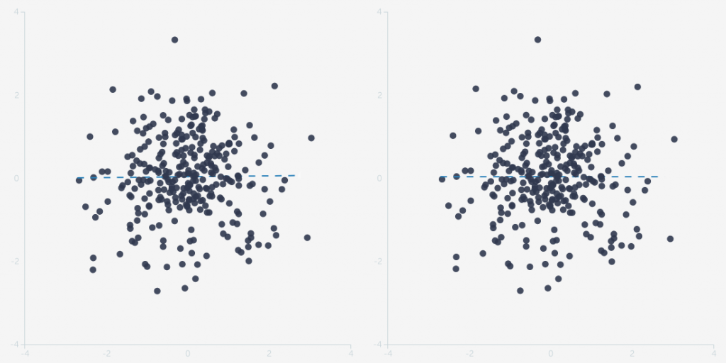
Experiments 3 and 4 lack any sort of control, so we’re left to consider the strongest pair of experiments in Bem’s paper, 8 and 9. Bem used a Differential Recall score instead of the raw guess count, as it makes the null effect have an expected value of zero. This Bayesian analysis can cope with a non-zero null, so I’ll just use a conventional success/failure count.

Experiments 8 and 9 from Bem's 2011 paper.

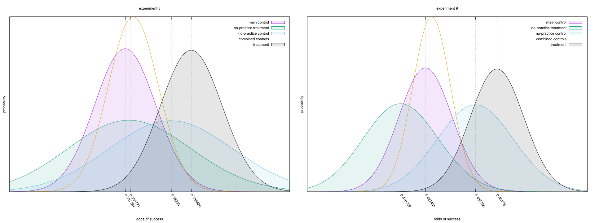
On the surface, everything’s on the up-and-up. The controls have more datapoints between them than the treatment group, but there’s good and consistent separation between them and the treatment. Look very careful at the numbers on the bottom, though; the effects are in quite different places. That’s strange, given the second study only differs from the first via some extra practice (page 14); I can see that improving up the main control and treatment groups, but why does it also drag along the no-practice groups? Either there aren’t enough samples here to get rid of random noise, which seems unlikely, or the methodology changed enough to spoil the replication.

Come to think of it, one of those controls isn’t exactly a control. I’ll let Bem explain the difference.

Participants were first shown a set of words and given a free recall test of those words. They were then given a set of practice exercises on a randomly selected subset of those words. The psi hypothesis was that the practice exercises would retroactively facilitate the recall of those words, and, hence, participants would recall more of the to-be-practiced words than the unpracticed words. […]

Although no control group was needed to test the psi hypothesis in this experiment, we ran 25 control sessions in which the computer again randomly selected a 24-word practice set but did not actually administer the practice exercises. These control sessions were interspersed among the experimental sessions, and the experimenter was uninformed as to condition. [page 13]

So the “no-practice treatment,” as I dubbed it in the charts, is actually a test of precognition! It happens to be a lousy one, as without a round of post-hoc practice to prepare subjects their performance should be poor. Nonetheless, we’d expect it to be as good or better than the matching controls. So why, instead, was it consistently worse? And not just a little worse, either; for experiment 9, it was as worse from its control as the main control was from its treatment group.

What it all Means

I know, I seems to be a touch obsessed with one social science paper. The reason has less to do with the paper than the context around it: you can make a good argument that the current reproducibility crisis is thanks to Bem. Take the words of E.J. Wagenmakers et al.

Instead of revising our beliefs regarding psi, Bem’s research should instead cause us to revise our beliefs on methodology: The field of psychology currently uses methodological and statistical strategies that are too weak, too malleable, and offer far too many opportunities for researchers to befuddle themselves and their peers. […]

We realize that the above flaws are not unique to the experiments reported by Bem (2011). Indeed, many studies in experimental psychology suffer from the same mistakes. However, this state of affairs does not exonerate the Bem experiments. Instead, these experiments highlight the relative ease with which an inventive researcher can produce significant results even when the null hypothesis is true. This evidently poses a significant problem for the field and impedes progress on phenomena that are replicable and important.

Wagenmakers, Eric–Jan, et al. “Why psychologists must change the way they analyze their data: the case of psi: comment on Bem (2011).” (2011): 426.

When it was pointed out Bayesian methods wiped away his results, Bem started doing Bayesian analysis. When others pointed out a meta-analysis could do the same, Bem did that too. You want open data? Bem was a hipster on that front, sharing his data around to interested researchers and now the public. He’s been pushing for replication, too, and in recent years has begun pre-registering studies to stem the garden of forking paths. Bem appears to be following the rules of science, to the letter.

I also know from bitter experience that any sufficiently large research project will run into data quality issues. But, now that I’ve looked at Bem’s raw data, I’m feeling hoodwinked. I expected a few isolated issues, but nothing on this scale. If Bem’s 2011 paper really is a type specimen for what’s wrong with the scientific method, as practiced, then it implies that most scientists are garbage at designing experiments and collecting data.

I’m not sure I can accept that.

How to Become a Radical

If I had a word of the week, it would be “radicalization.” Some of why the term is hot in my circles is due to offline conversations, some of it stems from yet another aggrieved white male engaging in terrorism, and some from yet another study confirms Trump voters were driven by bigotry (via fearing the loss of privilege that comes from giving up your superiority to promote equality).

Some just came in via Rebecca Watson, though, who pointed me to a fascinating study.

For example, a shift from ‘I’ to ‘We’ was found to reflect a change from an individual to a collective identity (…). Social status is also related to the extent to which first person pronouns are used in communication. Low-status individuals use ‘I’ more than high-status individuals (…), while high-status individuals use ‘we’ more often (…). This pattern is observed both in real life and on Internet forums (…). Hence, a shift from “I” to “we” may signal an individual’s identification with the group and a rise in status when becoming an accepted member of the group.

… I think you can guess what Step Two is. Walk away from the screen, find a pen and paper, write down your guess, then read the next paragraph.

The forum investigated here is one of the largest Internet forums in Sweden, called Flashback (…). The forum claims to work for freedom of speech. It has over one million users who, in total, write 15 000 to 20 000 posts every day. It is often criticized for being extreme, for example in being too lenient regarding drug related posts but also for being hostile in allowing denigrating posts toward groups such as immigrants, Jews, Romas, and feminists. The forum has many sub-forums and we investigate one of these, which focuses on immigration issues.

The total text data from the sub-forum consists of 964 Megabytes. The total amount of data includes 700,000 posts from 11th of July, 2004 until 25th of April, 2015.

How did you do? I don’t think you’ll need pen or paper to guess what these scientists saw in Step Three.

We expected and found changes in cues related to group identity formation and intergroup differentiation. Specifically, there was a significant decrease in the use of ‘I’ and a simultaneous increase in the use of ‘we’ and ‘they’. This has previously been related to group identity formation and differentiation to one or more outgroups (…). Increased usage of plural, and decreased frequency of singular, nouns have also been found in both normal, and extremist, group formations (…). There was a decrease in singular pronouns and a relative increase in collective pronouns. The increase in collective pronouns referred both to the ingroup (we) and to one or more outgroups (they). These results suggest a shift toward a collective identity among participants, and a stronger differentiation between the own group and the outgroup(s).

Brilliant! We’ve confirmed one way people become radicalized: by hanging around in forums devoted to “free speech,” the hate dumped on certain groups gradually creates an in-group/out-group dichotomy, bringing out the worst in us.

Unfortunately, there’s a problem with the staircase.

Categories Dictionaries Example words Mean r
Group differentiation First person singular I, my, me -.0103 ***
First person plural We, our, us .0115 ***
Third person plural They, them, their .0081 ***
Certainty Absolutely, sure .0016 NS

***p < .001. NS = not significant. n=11,751.

Table 2 tripped me up, hard. I dropped by the ever-awesome R<-Psychologist and cooked up two versions of the same dataset. One has no correlation, while the other has a correlation coefficient of 0.01. Can you tell me which is which, without resorting to a straight-edge or photo editor?

Comparing two datasets, one with r=0, the other with r=0.01.

I can’t either, because the effect size is waaaaaay too small to be perceptible. That’s a problem, because it can be trivially easy to manufacture a bias at least that large. If we were talking about a system with very tight constraints on its behaviour, like the Higgs Boson, then uncovering 500 bits of evidence over 2,500,000,000,000,000,000 trials could be too much for any bias to manufacture. But this study involves linguistics, which is far less precise than the Standard Model, so I need a solid demonstration of why this study is immune to biases on the scale of r = 0.01.

The authors do try to correct for how p-values exaggerate the evidence in large samples, but they do it by plucking p < 0.001 out of a hat. Not good enough; how does that p-value relate to studies of similar subject matter and methodology? Also, p-values stink. Also also, I notice there’s no control sample here. Do pro-social justice groups exhibit the same trend over time? What about the comment section of sports articles? It’s great that their hypotheses were supported by the data, don’t get me wrong, but it would be better if they’d tried harder to swat down their own hypothesis. I’d also like to point out that none of my complaints falsify their hypotheses, they merely demonstrate that the study falls well short of confirmed or significant, contrary to what I typed earlier.

Alas, I’ve discovered another path towards radicalization: perform honest research about the epistemology behind science. It’ll ruin your ability to read scientific papers, and leave you in despair about the current state of science.

Bayes Bunny iz trying to cool off after reading too many scientific papers.

One Hundred Prisoners

Here’s a question to puzzle out:

An especially cruel jailer announces a “game” to their 100 prisoners. A cabinet with 100 drawers sits in a heavily-monitored room. In each drawer lies one prisoner’s number. If every prisoner draws their own number from a drawer, every one of them walks free; if even one of them fails, however, all the prisoners must spend the rest of their days in solitary confinement. Prisoners must reset the drawers and room after their attempt, otherwise all of them head to solitary, and to ensure they cannot give each other hints everyone goes directly to solitary after their attempt. The jailer does offer a little mercy, though: prisoners can check up to half the drawers in the cabinet during their attempt, and collectively they have plenty of time to brainstorm a strategy.

What is the best one they could adopt?

This seems like a hopeless situation, no doubt. The odds of any one prisoner randomly finding their number is 50%, and the odds of that happening 100 times are so low they make death by shark look like a sure thing.

Nonetheless, the prisoners settle on a strategy. With a little programming code, we can evaluate the chances it’ll grant all their freedom.

      Algorithm	    Trials	      Successes	Percentage
   Random Guess	     50000	              0	0.0000000
         Cyclic	     50000	          15687	31.3740000

Whhaaa? How can the prisoners pull off odds like that? [Read more…]

Model Failure

This may be hard to believe, but I’m not about to talk about Bayesian modeling nor CompSci. Nope, I got dragged into an argument over implicit bias with a science-loving “skeptic,” and a few people mobbed me over the “model minority.”

Asian-Americans, like Jews, are indeed a problem for the “social-justice” brigade. I mean, how on earth have both ethnic groups done so well in such a profoundly racist society? How have bigoted white people allowed these minorities to do so well — even to the point of earning more, on average, than whites? Asian-Americans, for example, have been subject to some of the most brutal oppression, racial hatred, and open discrimination over the years. In the late 19th century, as most worked in hard labor, they were subject to lynchings and violence across the American West and laws that prohibited their employment. They were banned from immigrating to the U.S. in 1924. Japanese-American citizens were forced into internment camps during the Second World War, and subjected to hideous, racist propaganda after Pearl Harbor. Yet, today, Asian-Americans are among the most prosperous, well-educated, and successful ethnic groups in America. What gives?

What gives is simple demographics. Take it away, Jeff Guo of the Washington Post: [Read more…]

Fake Hate, Frequentism, and False Balance

This article from Kiara Alfonseca of ProPublica got me thinking.

Fake hate crimes have a huge impact despite their rarity, said Ryan Lenz, senior investigative writer for the Southern Poverty Law Center Intelligence Project. “There aren’t many people claiming fake hate crimes, but when they do, they make massive headlines,” he said. It takes just one fake report, Lenz said, “to undermine the legitimacy of other hate crimes.”

My lizard brain could see the logic in this: learning one incident was a hoax opened up the possibility that others were hoaxes too, which was comforting if I thought that world was fundamentally moral. But with a half-second more thought, that view seemed ridiculous: if we go from a 0% hoax rate to 11% in our sample, we’ve still got good reason to think the hoax rate is low.

With a bit more thought, I realized I had enough knowledge of probability to determine who was right.

[Read more…]

P-values are Bullshit, 1942 edition

I keep an eye out for old criticisms of null hypothesis significance testing. There’s just something fascinating about reading this…

In this paper, I wish to examine a dogma of inferential procedure which, for psychologists at least, has attained the status of a religious conviction. The dogma to be scrutinized is the “null-hypothesis significance test” orthodoxy that passing statistical judgment on a scientific hypothesis by means of experimental observation is a decision procedure wherein one rejects or accepts a null hypothesis according to whether or not the value of a sample statistic yielded by an experiment falls within a certain predetermined “rejection region” of its possible values. The thesis to be advanced is that despite the awesome pre-eminence this method has attained in our experimental journals and textbooks of applied statistics, it is based upon a fundamental misunderstanding of the nature of rational inference, and is seldom if ever appropriate to the aims of scientific research. This is not a particularly original view—traditional null-hypothesis procedure has already been superceded in modern statistical theory by a variety of more satisfactory inferential techniques. But the perceptual defenses of psychologists are particularly efficient when dealing with matters of methodology, and so the statistical folkways of a more primitive past continue to dominate the local scene.[1]

… then realising it dates from 1960. So far I’ve spotted five waves of criticism: Jerzy Neyman and Egon Peterson head the first, dating from roughly 1928 to 1945; a number of authors such as the above-quoted Rozeboom formed a second wave between roughly 1960 and 1970; Jacob Cohen kicked off a third wave around 1990, which maybe lasted until his death in 1998; John Ioannidis spearheaded another wave in 2005, though this died out even quicker; and finally the “replication crisis” that kicked off in 2011 and is still ongoing as I type this.

I do like to search for papers outside of those waves, however, just to verify the partition. This one doesn’t qualify, but it’s pretty cool nonetheless.

Berkson, Joseph. “Tests of Significance Considered as Evidence.” Journal of the American Statistical Association 1942;37:325-35. International Journal of Epidemiology, vol. 32, no. 5, 2003, pp. 687.

For instance, they point to a specific example drawn from Ronald Fisher himself. The latter delves into a chart of eye facet frequency in Drosophila melanogaster, at various temperatures, and extracts some means. Conducting an ANOVA test, Fisher states “deviations from linear regression are evidently larger than would be expected, if the regression were really linear, from the variations within the arrays,” then concludes “There can therefore be no question of the statistical significance of the deviations from the straight line.”

Berkson’s response is to graph the dataset.eye facets vs. temperature, Drosophila Melangaster, graphed and fit to a line. From Fisher (1938).

The middle points look like outliers, but it’s pretty obvious we’re dealing with a linear relationship. That Fisher’s tests reject linearity is a blow against using them.

Jacob Cohen made a very strong argument against Fisherian frequentism in 1994, the “permanent illusion,” which he attributes to a paper by Gerd Gigerenzer in 1993.[3][4] I can’t find any evidence Gigerenzer actually named it that, but it doesn’t matter; Berkson scoops both of them by a whopping 51 years, then extends the argument.

Suppose I said, “Albinos are very rare in human populations, only one in fifty thousand. Therefore, if you have taken a random sample of 100 from a population and found in it an albino, the population is not human.” This is a similar argument but if it were given, I believe the rational retort would be, “If the population is not human, what is it?” A question would be asked that demands an affirmative answer. In the hull hypothesis schema we are trying only to nullify something: “The null hypothesis is never proved or established but is possibly disproved in the course of experimentation.” But ordinarily evidence does not take this form. With the corpus delicti in front of you, you do not say, “Here is evidence against the hypothesis that no one is dead.” You say, “Evidently someone has been murdered.”[5]

This hints at Berkson’s way out of the p-value mess: ditch falsification and allow evidence in favour of hypotheses. They point to another example or two to shore up their case, but can’t extend this intuition to a mathematical description of how this would work with p-values. A pity, but it was for the best.


[1] Rozeboom, William W. “The fallacy of the null-hypothesis significance test.” Psychological bulletin 57.5 (1960): 416.

[2] Berkson, Joseph. “Tests of Significance Considered as Evidence.” Journal of the American Statistical Association 1942;37:325-35. International Journal of Epidemiology, vol. 32, no. 5, 2003, pp. 687.

[3] Cohen, Jacob. “The Earth is Round (p < .05).” American Psychologist, vol. 49, no. 12, 1994, pp. 997-1003.

[4] Gigerenzer, Gerd. “The superego, the ego, and the id in statistical reasoning.” A handbook for data analysis in the behavioral sciences: Methodological issues (1993): 311-339.

[5] Berkson (1942), pg. 326.

Stat of the Union

Time to do another deep dive on polling in the US. The first item comes via Steven Rosenfeld over at AlterNet. A number of polling companies have examined Trump’s standing in swing states, and compared it to how they voted. Their findings? They like him more than the average American, but less than when they voted for him. As Chuck Todd/Mark Murray/Carrie Dann put it at MSNBC,

In the Trump “Surge Counties” — think places like Carbon, Pa., which Trump won, 65%-31% (versus Mitt Romney’s 53%-45% margin) — 56% of residents approve of the president’s job performance. But in 2016, Trump won these “Surge Counties” by a combined 65%-29%. And in the “Flip Counties” — think places like Luzerne, Pa., which Obama carried 52%-47%, but which Trump won, 58%-39% — Trump’s job rating stands at just 44%. Trump won these “Flip Counties” by a combined 51%-43% margin a year ago.

So the sagging of support I mentioned a few months ago continues to happen. Rosenfeld also links to a few interviews with Trump voters, to get a more qualitative idea of where they’re at. There’s no real change there, they have a pessimistic view of what he’ll accomplish but praise him as a disruptor in fairly irrational terms. Take Ellen Pieper.

Poll respondent Ellen Pieper is among those disapproving of the president’s performance so far. The independent from Waukee voted for Trump and said she still believes in his ideas and qualifications. It’s how he behaves that bothers her. “He’s trying to move the country in the right direction, but his personality is getting in the way,” she said, calling out his use of Twitter in particular. “He’s a bright man, and I believe he has great ideas for getting the country back on track, but his approach needs some polish.”

Still, Pieper says, she’d vote for him again today.

Rosenfeld also makes some interesting comparisons to Nixon, but you’ll have to click through for that.

The second item comes via G. Elliott Morris, who’s boosted some diagrams made by Ian McDonald as well as their own. [Read more…]

Russian Hacking and Bayes’ Theorem, Part 2

I think I did a good job of laying out the core hypotheses last time, save two: the Iranian government or a disgruntled Democrat did it. I think I can pick them up on-the-fly, so let’s skip ahead to step 2.

The Priors

What’s the prior odds of the Kremlin hacking into the DNC and associated groups or people?
I’d say they’re pretty high. Right back to the Bolshevik revolution, Russian spy agencies have taken an interest in running disinformation campaigns. They have a word for gathering compromising information to blackmail people into doing their bidding, “kompromat.” Putin himself earned a favourable place in Boris Yeltsin’s government via some kompromat of one of Yeltsin’s opponents.
As for hacking elections, European intelligence agencies have also fingered Russia for using kompromat to interfere with elections in Germany, the Netherlands, Hungary, Georgia, and Ukraine.
That’s all well and good, but what about other actors? China also has sophisticated information warfare capabilities, but they seem more interested in trade secrets and tend to keep their discoveries under wraps. North Korea is a lot more splashy, but recently have focused on financial crimes. The Iranian government has apparently stepped up their online attack capabilities, and have a grudge against the USA, but apparently focus on infrastructure and disruption.
The DNC convention was rather contentious, with fans of Bernie Sanders bitter at how it turned out, and putting Trump in power had been preferred to voting for Clinton, for some, but it doesn’t fit the timeline: the DNC was suspicious of an attack in April, documents were leaked in June, but Sanders still had a chance of winning the nomination until the end of July.
An independent group is the real wild card, with any number of motivations and due to their lack of power eager to make it look like someone else did the deed.
What about the CIA or NSA? The latter claims to be just a passive listener, and I haven’t heard of anyone claiming otherwise. The CIA has a long history of interfering in other countries’ elections; in 1990’s Nicaragua, they even released documents to the media in order to smear a candidate they didn’t like. It’s one thing to muck around with other countries, however, as it’ll be nearly impossible for them to extradite you over for a proper trial. Muck around in your own country’s election, and there’s no shortage of reporters and prosecutors willing to go after you.
Where does all this get us? I’d say to a tier of prior likelihoods:
  • “The Kremlin did it” (A) and “Independent hackers did it” (D) have about the same prior.
  • “China,” (B) “North Korea,” (C) “Iran,” (H) and “the CIA” (E) are less likely than the prior two.
  • “the NSA” (F) and “disgruntled insider” (I) is less likely still.
  • And c’mon, I’m not nearly good enough to pull this off. (G)

The Evidence

I haven’t placed quantities to the priors, because the evidence side of things is pretty damning. Let’s take a specific example: the Cyrillic character set found in some of the leaked documents. We can both agree that this can be faked: switch around the keyboard layout, plant a few false names, and you’re done. Do it flawlessly and no-one will know otherwise.
But here’s the kicker: is there another hypothesis which is more likely than “the Kremlin did it,” on this bit of evidence? To focus on a specific case, is it more likely that an independent hacking group would leave Cyrillic characters and error messages in those documents than Russian hackers? This seems silly; an independent group could leave a false trail pointing to anyone, which dilutes the odds of them pointing the finger at a specific someone. Even if the independent group had a bias towards putting the blame on Russia, there’s still a chance they could finger someone else.
Put another way, a die numbered one through six could turn up a one when thrown, but a die with only ones on each face would be more likely to turn up a one. A one is always more likely from the second die. By the same token, even though it’s entirely plausible that an independent hacking group would switch their character sets, the evidence still provides better proof of Russian hacking.
What does evidence that points away from the Kremlin look like?

President Vladimir Putin says the Russian state has never been involved in hacking.

Speaking at a meeting with senior editors of leading international news agencies Thursday, Putin said that some individual “patriotic” hackers could mount some attacks amid the current cold spell in Russia’s relations with the West.
But he categorically insisted that “we don’t engage in that at the state level.”

Is this great evidence? Hell no, it’s entirely possible Putin is lying, and given the history of KGB and FSB it’s probable. But all that does is blunt the magnitude of the likelihoods, it doesn’t change their direction. By the same token, this ….
Intelligence agency leaders repeated their determination Thursday that only “the senior most officials” in Russia could have authorized recent hacks into Democratic National Committee and Clinton officials’ emails during the presidential election.
Director of National Intelligence James Clapper affirmed an Oct. 7 joint statement from 17 intelligence agencies that the Russian government directed the election interference…
….  counts as evidence in favour of the Kremlin being the culprit, even if you think James Clapper is a dirty rotten liar. Again, we can quibble over how much it shifts the balance, but no other hypothesis is more favoured by it.
We can carry on like this through a lot of the other evidence.
I can’t find anyone who’s suggested North Korea or the NSA did it. The consensus seems to point towards the Kremlin, and while there are scattered bits of evidence pointing elsewhere there isn’t a lot of credibility or analysis attached, and some of it is “anyone but Russia” instead of “group X,” which softens the gains made by other hypotheses.
The net result is that the already-strong priors for “the Kremlin did it” combine with the direction the evidence points in, and favour that hypothesis even more. How strongly it favours that hypothesis depends on how you weight the evidence, but you have to do some wild contortions to put another hypothesis ahead of it. A qualitative analysis is all we need.
Now, to some people this isn’t good enough. I’ve got two objections to deal with, one from Sam Biddle over at The Intercept, and another from Marcus Ranum at stderr. Part three, anyone?